II. Toward Carrollian Quantum Gravity

Trying to combine GR and QM in a way that doesn't assume the Planck length

Introduction

The motivation for this post can be found in the previous one. The TL; DR is that I argued you can’t just smash together General Relativity (GR, containing fundamental constants G and c) and Quantum Field Theory (QFT, containing fundamental constants ℏ and c) without it immediately sending you down the path of a Planck length-based take on Quantum Gravity (QG). Using G, c, and ℏ to make ℓₚ = √Gℏ/c³ may in fact be the correct route to QG — but like string theory it has been 50+ years with no real progress¹.

My suggestion was to instead treat G, c, and ℏ as a “pick two” trilemma and see what happens when you pick G and ℏ in order to complete the triangle. At the classical level, there are two theories (symmetry algebras) that are dual to each other when you use the two different limits to remove c from the Poincaré symmetry of Minkowski space: the Galilean limit (c → ∞) and the Carrollian limit (c → 0). While non-relativistic quantum gravity via the Galilean limit is a possible route (see e.g. here), I argued in the previous post that Carrollian Quantum Gravity (CQG) might be the more fruitful approach.

Preliminaries

Spacetime in the Carrollian limit consists of a “somenified” manifold with degenerate covariant spacelike metric hᵢⱼ and trivial contravariant timelike “metric” ξⁱ ξʲ made from Killing vectors ξⁱ. Carrollian time s has units of L²/T to keep the duality with the Galilean limit manifest, and, per the quantum speed limit of the previous post, can be set by a scale ℏ/m where m is the mass of a stationary particle with spin J. There is a scalar complex tachyon field σ that will be discussed below.

First, we are assuming non-relativistic quantum mechanics (NRQM, so we have ℏ) and non-relativistic gravity — at least the existence of the fundamental physical constant G. The (G , ℏ) side is the side of the “pick two” trilemma triangle we are expanding from to try to build CQG. The Carrollian limit means we do not have a fundamental constant c. However, since you cannot send a dimensionful constant like c to zero in physics without a lot of handwaving, we will use a “loophole” from the previous post — we assume a vacuum energy density² and a suitable energy condition so that we have a speed of sound vₛ² = dP/dρ for complex scalar excitations (field σ) propagating in that energy density (see the previous post for more details). The Carrollian limit is then c ≪ vₛ.

Second, there are three representations of the Lorentz group “allowed” in QFT: 1. massive particles with definite momentum and spin that travel slower than c (e.g. electrons), 2. massless particles with definite momentum and helicity (“momentum dot spin”) that travel at c (e.g. photons), and 3. spinless (spin zero) tachyons with definite momentum that travel faster than c (e.g. the pre-electroweak symmetry breaking Higgs boson). Since anything that propagates through space in the Carrollian limit is by definition a tachyon, we basically have two things in our theory: tachyons and stationary massive particles. Since tachyons have zero energy in the Carrollian limit (see here³), they are “soft” in the sense of the relationship between soft theorems and asymptotic symmetries — as a complex scalar field σ quanta would represent a complex number phase change ∈ U(1) of the vacuum state.

Third is the “quantum speed limit”. In a Carrollian spacetime, we have

\(\displaystyle s \geq s^{Q} = \frac{\pi}{2} \frac{\hbar}{m}\)

Our (immobile) quantum states with mass m can transition from one state to a distinguishable orthogonal one in a Carrollian time no faster than sꟴ which sets the limit of the quantum state’s internal “clock”. Now this is where our assumptions run up against the “problem of time” in QG — i.e. our assumptions here may imply a particular view of the problem of time⁴. I have not worked through the philosophy in detail⁵, but let’s make an assumption that gives us consistency with special relativity. In the frame of the particle the clock ticks⁶ in units of sꟴ tick at a rate as they would in flat space⁷. So while a large system with mass M ≫ m would experience its own clock ticking normally in its own frame, an observer with mass m would see only small increments of Δs ~ ℏ/M pass while they (the observer) zipped forward along the (Carrollian) time axis in increments of ~ ℏ/m ≫ ℏ/M. We’re like 90% of the way to the view of gravity in the weak field limit in GR at this point, so let’s get into the primary objective.

Carrollian Quantum Gravity: A First Draft

Most labels are as in the previous diagram. Very massive system with mass M ≫ m propagates forward in time in “clock” steps ~ ℏ/M acquiring a quantum phase φ which excites the tachyon field σ with a quantum that propagates at vₛ ≫ c carrying the opposite phase (i.e. net phase change of M plus vacuum = 0) to another (test) particle of mass m. I left it off the diagram but the two systems m and M are a distance R apart on a spacelike slice Σ.

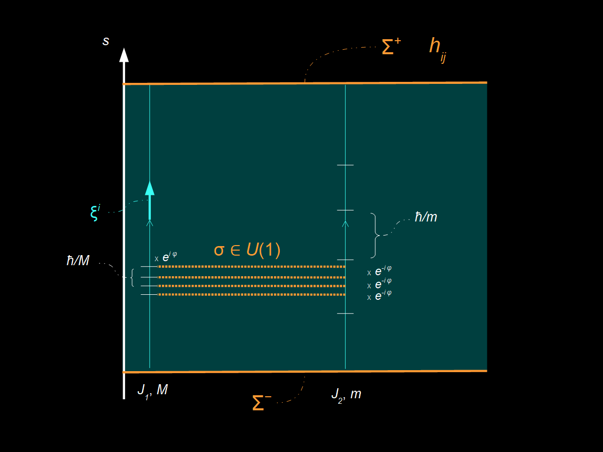
Ok. Last assumption. We have a large⁸ mass system with mass M. For it, Δs ~ ℏ/M and each “clock step” carries it forward in Carrollian time with an added⁹ phase exp(+𝒾 φ). We assume this is accompanied by an excitation of the complex scalar tachyon field carrying the opposite phase ~ exp(−𝒾 φ) as a kind of “conservation of phase”. The phase shift of the test mass state would then be:

\(\displaystyle \begin{eqnarray} +\frac{i}{\hbar} m \, \delta s -i \varphi & = & \frac{i}{\hbar} m \, \delta s-\frac{i}{\hbar} E \frac{\delta s}{v_{s}^{2}}\\ &=& \frac{i}{\hbar} m \frac{\pi}{2} \frac{\hbar}{m} - \frac{i}{\hbar} E \frac{\pi}{2} \frac{\hbar}{m \, v_{s}^{2}}\\ &=&i\frac{\pi}{2}\left(1 - \frac{E}{m v_{s}^{2}} \right) \end{eqnarray}\)

Of course, to really work as a conservation law the phase needs to approach 2πn for n ∈ ℤ at a rate ~1/R in energy¹⁰. There are probably lots of ways we could try to understand that energy E, but the easy one given the assumptions is that it is the non-relativistic gravitational potential energy ~ G Mm/R. So as our mass M moves forward in time by a clock step in its own frame, the test mass a distance R away is “dragged back¹¹ in time” due to a tachyon exchange by a factor

\(\displaystyle \begin{eqnarray} 1 - \frac{E}{m v_{s}^{2}} & = & 1 - \frac{G M m}{R \; m v_{s}^{2}}\\ & = & 1 - \frac{G M}{R \; v_{s}^{2}}\\ & = & 1 - \frac{R_{0}}{R} \end{eqnarray}\)

where R₀ ≡ G M/vₛ² which is, up to a factor¹² of 2, the Schwarzschild radius if vₛ = c. (I should also note that if vₛ = c we can recover w = −1 and the ordinary cosmological constant.) Another test mass nearby would experience a tiny differential “time dilation”. If the two test mass systems were connected, there would be a 4-velocity torque bending the coupled system towards M with increasing velocity (i.e acceleration) as time marched forward. However, we are in the Carrollian limit so nothing can move. It can only feel the pull of what is essentially gravity slowing its internal clock — geodesics that would curve due to the curvature of time¹³ but can’t.

This time dilation effect really is gravity! At least in our ultra-local Carrollian limit that’s dual to the non-relativistic Galilean limit. There are quite a few avenues to explore from this simple “Carrollian Quantum Gravity” baseline. The exchange of these scalar tachyons would entangle the particles so there are some entropy calculations to be done. There’s also a way to create a “light cone” using unitary operators in a quantum circuit¹⁴. That might be helpful in understanding “black holes” (i.e. a test mass falling inside a region R < G M/vₛ² ) in this model CQG.

Now you might be uncomfortable with the tachyons. They’re weird. The approach I am presenting is basically dependent on a bunch of loopholes from energy conditions to allowed representations of the Lorentz group. But it’s not like these loopholes haven’t been used before! The Higgs boson is a tachyon field. Sure we don’t live in its “unstable” tachyon phase with unbroken SU(2) electroweak symmetry, but then the Carrollian limit isn’t exactly our everyday experience either. We’re also talking about “events” happening elsewhere from the point of view of any observer in Carrollian spacetime. Per the previous post, it would be an extension our view of causality to impose causal physics in regions of spacetime we don’t have access to. Plus what about “spooky action at a distance”? It empirically exists in manifestly Lorentz invariant quantum field theory, so I’d think it was a conservative view to give it a speed limit ~ vₛ. However the most intuitive view for me is the quantum circuit view — those gates are tachyons in the way they’re typically depicted. The picture above is essentially a mathematically coherent way of having qubits operating at different “clock speeds” and relating them via logic gates that are just a phase¹⁵.

Of course this is a blog post so hasn’t been peer reviewed. There’s not even all that much here besides setting up a system and exploring a couple of consequences of assumptions. Also — while I feel like I’ve done a reasonable literature search it is entirely possible I’ve missed someone who as done this before¹⁶. All I know is that this is not a common take on combining quantum mechanics and gravity. And it doesn’t assume the Planck length¹⁷! That was the primary goal.

Update 4 July 2025

Wanted to add that the gravitational time dilation we arrived at above is the leading order effect:

\(\displaystyle \begin{eqnarray} t' \simeq t \sqrt{1 - \frac{2 G M}{R \, v_{s}^{2}}} & \approx & t - t \frac{ G M}{R \, v_{s}^{2}} + o(G^{2})\\ & = & t \left( 1 - \frac{ G M}{R \, v_{s}^{2}}\right)\\ & = & t \left( 1 - \frac{ R_{0}}{R}\right) \end{eqnarray}\)

where I kept it in terms of vₛ² instead of c² as would be the case in ‘normal’ GR (and R₀ is the Schwarzschild radius) that is recovered in the limit vₛ ≈ c.

I also wanted to add that the phase of the large mass M changes by

\(\displaystyle \begin{eqnarray} + i \varphi & = & \frac{i}{\hbar} M \, v_{s}^{2}\, \frac{\delta s}{v_{s}^2}\\ & \simeq & \frac{i}{\hbar} M \, \frac{\pi}{2} \frac{\hbar}{M}\\ & = & i \frac{\pi}{2} \end{eqnarray}\)

which is just the “phase rotation into an orthogonal state” per the quantum speed limit. This is the analogous first term in the calculation with the smaller mass above.

1. As noted in the previous post, the progress that has occurred has been centered around possible consistent resolutions of problems incurred by starting with the Planck length. (E.g. the black hole information paradox.)

2. Oh hey — this is a real thing: ρ = Λ c²/8πG. Some minor issues with the Carrollian limit, but they work out (see here).

3. Note: this paper does not adopt the Carrollian time units used in this post, and instead treats it as an ordinary time. I did work through all the math presented here using that convention and it works out, so while it is a preference thing it does help my intuition to use [s] = L²/T which has the benefit of making the duality between the Carrollian and Galilean limits manifest.

4. I’ll save discussion of this for later — when I feel like I have a handle on it myself.

5. I swear I am reading it though!

6. There are a lot of places you can go with this, but in a sense we are looking at a quantum computer with “tachyon” gates.

7. Interestingly since sꟴ ~ 1/m this would require a nonzero cosmological constant Λ to use as a clock reference for what we mean by flat space mass-energy in the absence of a mass m. Otherwise the minimum clock step is infinitely long!

8. This is mostly so we can neglect the tachyons on the opposite path from test mass m to M.

9. Going to work with the convention that “plus” is forward in time.

10. Technically the tachyons carry zero energy but we think of them in the sense of “soft” scalars maintaining asymptotic symmetries. Also remember Σ is still a 3D spacelike slice which is why force needs to fall ~ 1/R² and potential ~ 1/R instead of different exponents.

11. More “slowed in its progress forward in time”.

12. Though see via the update that the “missing” factor of 2 is also something that disappears in the expansion for small G (or technically R₀/R ≪ 1). The effective shrinking of the time interval is exactly equal to the leading order gravitational time dilation if vₛ = c.

13. The contribution of spatial curvature to the gravitational force we experience every day is actually relativity small (by factors of order 1/c²) compared to the “time curvature” component.

14. Teasing a diagram for a future post (adapted from this YouTube lecture from Strings 2019):

15. I just now realized this could have applications to quantum computing. Though can’t imagine off the top of my head why you’d want some qubits to move to orthogonal states faster than others. Just make them all clock at the fastest rate.

16. The footnote with the diagram above is taken from somewhere (I’ve seen this exact same or a similar picture in multiple places); when I find the reference I will link. It’s here (YouTube lecture from Strings 2019).

17. You could construct ℓ = √Gℏ/vₛ³ but ℓₚ ≫ ℓ so effectively ℓ ~ 0 and there is no minimal length scale.