Elsewhere and indivisible stochastic processes

A continuation of an earlier post

Introduction

In an earlier post, I talked about “quantum weirdness” and a new approach from Jacob Barandes (e.g. here) that seemed to mesh well with my crackpot take (here, here) that the fundamental uncertainty of Quantum Mechanics (QM) and the fundamental lack of knowledge of events that occur “elsewhere” in a spacetime diagram (i.e. at spacelike separation) are in fact the same loss of information. An indivisible stochastic process, i.e. that

\(\Gamma (t \leftarrow 0) \neq \Gamma(t \leftarrow t') \Gamma(t' \leftarrow 0) \)

for intermediate times t’, per Barandes, leads to much of the machinery of quantum mechanics. That indivisibility (I claim) is related to the system passing out of the observer’s light cone into the “elsewhere” region at time 0 and re-entering it at time t — or, more boldly, that QM = SR to paraphrase Susskind. Times t’ between 0 and t in a sense, um, do not make sense.

No sense of space

One thing about Barandes’ Indivisible Process (IP) reformulation of QM is that the only prima facie dimensionful content it has is time. In this paper, “energy” is added by hand through the ad hoc introduction of ℏ in defining the Hamiltonian:

\(H(t) \equiv i \hbar \frac{\partial U(t)}{\partial t} U^{\dagger}(t)\)

And since that time t is in fact the only dimensionful quantity, it could be replaced by an affine dimensionless parameter (e.g. rescale t → t/τ) WOLOG.

Since there’s only time, there’s no space and no speed of light c. That makes the treatment of the EPR thought experiment in his other paper a bit hand-wavy. We kind of have to assume there’s some operator on the set of configurations 𝒞 (Barandes’ notation) that produces a concept of spacetime distance. It’s actually a bit more vague than that: “The two observer subsystems A and B are assumed to remain spacelike separated throughout the experiment.” Or here: “The only causal influences on the observer-subsystem A are from the two [EPR-entangled] subsystems Q and R, which both intersect the past light cone of A.” Basically, the causal structure of Minkowski spacetime is assumed.

This is fine! Because I also want to assume Minkowski spacetime. I’ve reproduced his Figure 2 below:

Figure 2 from Barandes (2024) showing observer systems A and B. An EPR (Bell) state (Q,R) prepared at or prior to time t = 0 undergoes a transition at time t’ and the subsystems Q and R are measured as (A, Q) and (B,R) at time t. The trajectories of the EPR pair are shown despite not being an ontological component of Barandes’ interpretation.

Let me make a few suggestive edits to that diagram:

Figure 2 of Barandes (2024) with the assumed causal structure in the text made explicit (orange (brown?) past and future light cones of A and B), and removing the non-ontological trajectories. A classical communication from A to B is shown as a wavy line from after A’s observation of Q to the point where A and B’s light cones again intersect at time t. The common “elsewhere” region between A and B is where all the action happens.

Looks familiar! Of course, there’s no reason those EPR subsystems have to be relativistic, so we could remove observer B and just have A observe the two subsystems Q and R at different times:

The previous figure with observer system B removed and both products Q and R of the EPR state are observed by A. The right Rindler wedge is suggestively highlighted in teal. In the Rindler chart, there is a horizon between the brown and teal regions at Rindler time ± ∞ which the states (Q, R), Q, and R cross.

Barandes just needs an assumption that A and B have causal connection to (Q, R) and are spacelike separated until time t in order to make is EPR argument. This could be as simple as the basic aspects of special relativity in first lightcone diagram above, or B could be uniformly accelerated so that A and B are on opposite sides of a Rindler horizon as suggested by the second. Another way we could achieve this spacelike separation is by taking c → 0.

Carrollian limit

Taking the speed of light to zero (“Carrollian limit”) is the latest rage in theoretical physics. Per the paper in the previous link, the trigger point of the exponential rise in citations appears to be ~ 2014 when this paper was published which showed the BMS group (the symmetry of asymptotically flat Minkowski spacetime at null infinity) is the conformal extension of the Carroll algebra (contraction of the Poincare algebra c → 0). This opened the door to “flat space holography” (e.g. conference here). Previously physicists could only use anti-de Sitter (AdS) space with its unphysical negative curvature for explicit examples (e.g. AdS/CFT) of the holographic principle. Actual spacetime is (approximately) flat¹!

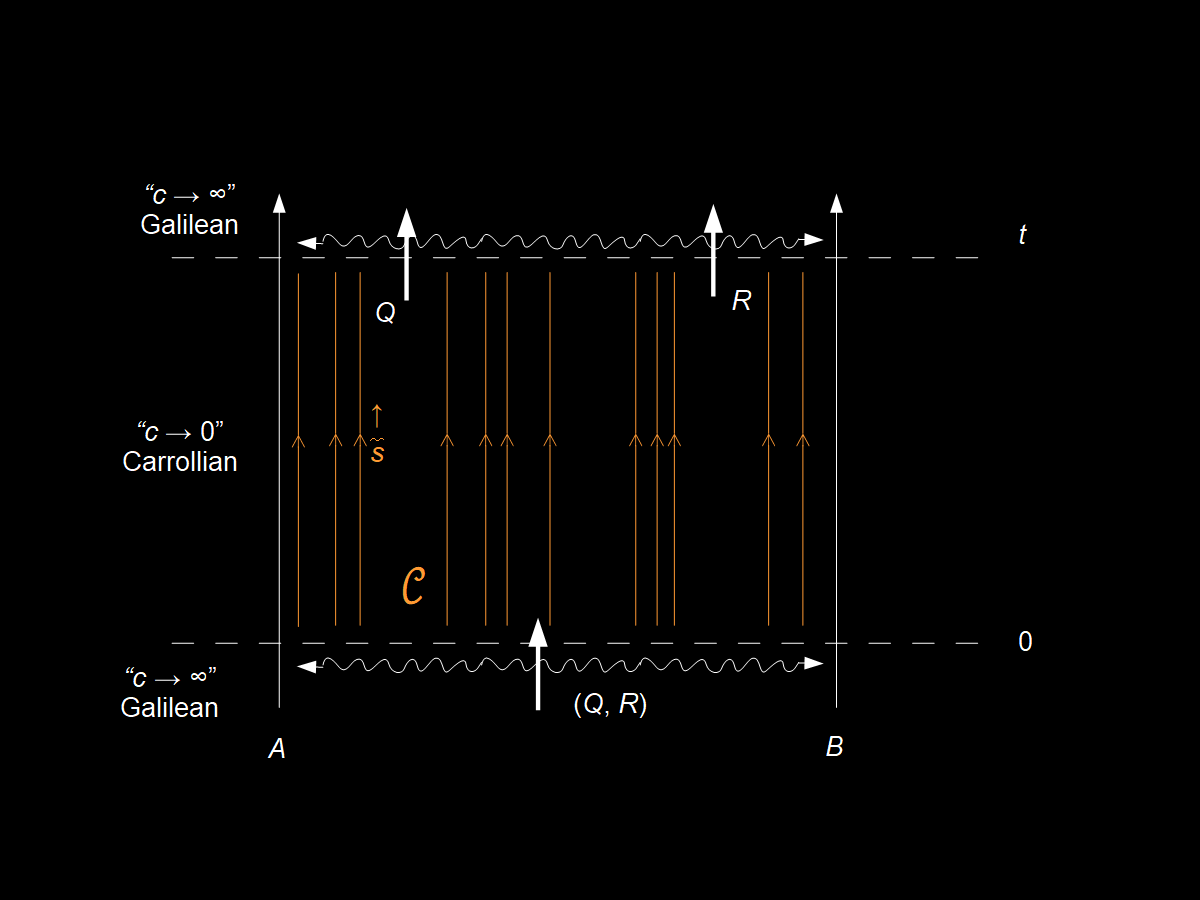
I had previously tinkered around with the Carrollian limit here, which closes up the observer light cones and makes every system stationary evolving along Carrollian time s. The “dynamics” as such are more about the changes in “configurations” in 𝒞 evolving over “time”. This picture is very much like the IP view in Barandes’ reformulation of QM during the period from 0 to t. I made a picture² where spacetime undergoes what I’m going to call a “bullet time” transformation³ such that c → c(t) where for [0,t] ⊂ (−∞, +∞) the function c(t) → 0 (Carrollian limit) and otherwise c(t) → +∞ (Galilean limit).

“Bullet time” transformation where the speed of light is “large” (infinite) before time 0 and after time t. This is indicated with horizontal light waves (wavy lines) representing classical communication between every subsystem after the experiment. Between 0 and t, the time of the experiment, the speed of light is “small” (zero). Configurations consisting of immobile “states” (orange lines) in 𝒞 evolve in Carrollian time s/(λ c).

I’ve made the Carrollian time s into a dimensionless quantity by introducing a length scale⁴ λ and a “velocity” v₀:

\(\tilde{s} = \frac{s}{\lambda \; v_{0}}\)

Instead of introducing ℏ (with units of energy times time) to make the units of the “Hamiltonian” time evolution operator for the indivisible stochastic process into energy as Barandes does, let’s create a dimensionless Carrollian time evolution operator

\(\tilde{K}(\tilde{s}) \equiv i \frac{\partial U(\tilde{s}) }{\partial \tilde{s}} U^{\dagger}(\tilde{s})\)

The 𝒾 is still necessary to make the operator Hermitian.

Bekenstein Bound

Now write the density matrix as a modular Hamiltonian

\(\rho(0) = \frac{e^{-\tilde{K}(0)}}{\text{tr} \; e^{-\tilde{K}(0)}}\)

Ostensibly ρ(0) doesn’t have any zero eigenvalues because we don’t have “traditional” quantum mechanics (or a fortiori quantum field theory) so there’s no such thing as a vacuum state — plus something (e.g. a particle) went in to our little patch of elsewhere. Therefore we can do that⁵.

Let’s evaluate a quantity I’m going to call ΔK

\(\begin{eqnarray} \Delta \tilde{K} & \equiv & \text{tr} \; \rho (\tilde{s}) \tilde{K}(0) - \text{tr} \; \rho (0) \tilde{K}(0) \\ & = & \text{tr} \; \rho (\tilde{s}) \left[ -\log \rho (0) - \log \text{tr} \; e^{-\tilde{K}(0)} \right] \\ & & - \text{tr} \; \rho (0) \left[ -\log \rho (0) - \log \text{tr} \; e^{-\tilde{K}(0)} \right] \\ & = & - \text{tr} \; \rho (\tilde{s}) \log \rho (0) + \text{tr} \; \rho (0) \log \rho (0) \\ & = & - \text{tr} \; \rho (\tilde{s}) \log \rho (0) - S(\rho (0)) \end{eqnarray}\)

where I’ve used

\(\begin{eqnarray} S(\rho) & \equiv & -\text{tr} \; \rho \log \rho \\ \text{tr} \; \rho & = & 1 \end{eqnarray}\)

along with inverting the modular Hamiltonian equation above. Let’s also evaluate⁶ ΔS

\(\begin{eqnarray} \Delta S & \equiv & S(\rho (\tilde{s})) - S(\rho (0))\\ & =& - \text{tr} \; \rho(\tilde{s}) \log \rho(\tilde{s}) + \text{tr} \; \rho(0) \log \rho(0) \end{eqnarray}\)

There is of course a known end point I am trying to get to (namely the title of this section), but let’s just write down the always non-negative relative entropy S(ρ|σ) ≥ 0

\(\begin{eqnarray} 0 \leq S(\rho(\tilde{s}) | \rho(0)) & = & \text{tr} \; \rho(\tilde{s}) \log \rho(\tilde{s}) - \text{tr} \; \rho(\tilde{s}) \log \rho(0)\\ & = & -S(\rho(\tilde{s})) - \text{tr} \; \rho(\tilde{s}) \log \rho(0)\\ &=& -S(\rho(\tilde{s})) + \Delta\tilde{K} + S(\rho(0))\\ & = & -\Delta S + \Delta\tilde{K}\\ & & \\ \rightarrow \Delta S & \leq & \Delta\tilde{K} \end{eqnarray}\)

We’ve basically followed Casini’s derivation of the Bekenstein bound. In that paper, K is a boost in the Rindler wedge and goes as ~ R E, which is dimensionless in natural units ℏ = c = 1 as that makes [R] = 1/E and [E] = E. There’s no “delta” but rather the background is subtracted because he was dealing with quantum field theory and the sums (traces) are generally divergent.

The other difference is that Casini was mostly using entanglement entropy (at least for the math, but went back and forth to thermodynamic entropy in the physical arguments). The spacetime region was broken into two pieces — one of which, V, was inside the Rindler wedge where all the action was happening. That means the traces are all done over complement of V (i.e. the rest of the universe) since

\(\rho_{V} = \text{tr}_{\bar{V}} \; \rho_{V \bar{V}}\)

which is intuitive mathematically but not physically (at least to me). I used good old-fashioned state counting of whatever degrees of freedom are behind the abstract configurations 𝒞 of the indivisible stochastic process inside V. It should be noted that it is not actually known what the right answer is here, and the answer will basically require quantum gravity (or some theory derived from indivisible stochastic processes).

A boost in the Carrollian limit is a Carrollian time, s, translation⁷:

\(\begin{eqnarray} s' & = & s + \textbf{v} \cdot \textbf{x}\\ \textbf{x}' & = & \textbf{x}\\ & \text{or} & \\ \tilde{s}' & = & \tilde{s} + \frac{\textbf{v} \cdot \textbf{x}}{v_{0} \; \lambda}\\ \textbf{x}' & = & \textbf{x} \end{eqnarray}\)

Which means the modular Hamiltonian is a boost! In fact, this is the Carrollian limit of the modular flow of the Rindler wedge:

Left: Modular flow in the Rindler wedge (teal). Following the curves is increasing Rindler time which is a boost transformation. Right: approaching the Carrollian limit where the observer’s light cone closes up (brown) and the Rindler wedge looks like the rest of Carrollian space with time parameter s going up.

Therefore if we back off from the Carrollian limit, we have something like

\(\begin{eqnarray} \Delta S & \lesssim & \lambda \; E\\ & \sim & \Delta x \; M \end{eqnarray}\)

which is Bousso’s covariant bound (see Eqn. 15), but offers yet another interpretation of the “size” R in Bekenstein’s bound. What “R” meant was something of a hand-wavy argument — with Bousso’s paper arguing it is the “smallest” dimension of an object. But now there is a connection to the de Broglie (or Compton) wavelength. Restoring the ℏ’s and c’s in Bousso’s bound we have:

\(\begin{eqnarray} \Delta S & \lesssim & \frac{\Delta x \; M c}{\hbar}\\ & = & \frac{ \Delta x}{\lambda} \end{eqnarray}\)

which is one way to count the particles of a system of “size” Δx, and as we approach S ~ 1, we are tantalizingly close to Bousso’s comment:

This remarkable fact suggests a novel perspective on the connection between gravity and quantum mechanics. Note that for systems with small numbers of quanta (S ≈ 1), Bekenstein’s bound can be seen to require non-vanishing commutators between conjugate variables, as they prevent Mx from becoming much smaller than ℏ. One is tempted to propose that at least one of the principles of quantum mechanics implicitly used in any verification of Bekenstein’s bound will ultimately be recognized as a consequence of Bekenstein’s bound, and thus of the covariant entropy bound and of the holographic relation it establishes between information and geometry.

Summary

What did we accomplish with all this hand-waving?

• There’s no “space” in Barandes’ IP formulation of QM, but there’s no “space” to speak of in the Carrollian limit either.

• There are no obvious inconsistencies if you assume “elsewhere” (SR) is the source of the lack of divisibility in the stochastic processes (QM).

• All of these things are consistent with the Bekenstein bound and in many ways “suggestive” of holography

1. Or even a little bit positive (positive cosmological constant) making it de Sitter (dS) space. But this presents its own problems.

2. Also made a more suggestive picture

where the symbols are the quantum circuit for preparing and measuring an EPR state.

3. There is a sense in which this is basically equivalent to a worldline (really a congruence for the whole system) that skirts a black hole for [0,t].

4. Actually, Carrollian time has dimensions of L²/T which is “action per mass” so I could have easily taken the constant to be ℏ / m — which if you set equal to λ v yields λ = ℏ / (m v) which is the de Broglie wavelength (or the Compton wavelength if v = c). However, I am trying to be somewhat agnostic right now. The reason Carrollian “time” has dimensions of L²/T is in order to make it a symmetric dual to the Galilean limit. Technically the “time” coordinate is the zero component of the 4-vector x⁰ (units of length!) so for our normal quasi-Galilean algebra with c very large you divide by c to get time t = x⁰/c. But for the dual Carrollian algebra has t = C x⁰ (yes capital C, not configurations with a script 𝒞) but still units of m/s).

5. Casini’s paper justifies this with the fact that the density matrix is just a subsystem in a region V, not the whole space, so doesn’t have the vacuum state and therefore no zero eigenvalues.

6. Wait — you ask. Isn’t this zero? It would be if this was actual quantum mechanics and ρ(s) was a unitary time evolution of ρ(0) with a time-independent Hamiltonian (yes this is redundant). Truthfully, we (well, I) cannot even assert it is positive for an indivisible stochastic process. The usual takes on the “entropy rate” for stochastic processes don’t really apply. The oscillatory example of an indivisible process (Eq. 16 in Barandes’ paper) has an entropy that, um, oscillates, so therefore for various values of “time” the entropy could be higher or lower than the initial state.

7. What’s super interesting (to me) is that the dimensionless s-tilde transformation can be seen as scaling the length (“de Broglie wavelength”) as if adjusting a coarse graining scale which is exactly like how some of the known mechanisms of emergent dimensions work. Translating along Carrollian time can be seen as changing wavelength as we go from “scri minus” ℐ ⁻ (past null infinity) at very short wavelength to the observer at long wavelength and back out to “scri plus” ℐ ⁺ (future null infinity) again at short wavelength.