More on the elsewhere interpretation of quantum mechanics

Carrollian limits and the appearance of Planck's constant

One of the more enjoyable aspects of having a sci fi blog is making up fake, but plausible, science. What’s more enjoyable than that? When your fake, but plausible science might not be fake.

My (limited) work on physics problems after leaving academia has mostly been relegated to hobbyist tinkering with fundamental questions — the kinds of things you only get paid to do if you’re Leonard Susskind or Andrew Strominger¹. Anyway, a year ago I laid out my lines of intuition behind what I’m calling “the elsewhere interpretation of quantum mechanics”:

I’d been tinkering with this for years. I have records that I talked about it via email with a grad school friend of mine back in 2010, and there’s probably other evidence since I remember he took a picture of my chalkboard in my apartment with the “Dirac” equation “derivation”² that I mention in the post linked above. There’s a fun side comment from Bousso in his covariant entropy bound paper (on which that “Dirac” equation “derivation” is based) that’s always been floating in the back of my head:

Note that for systems with small numbers of quanta (S ≈ 1), Bekenstein’s bound can be seen to require non-vanishing commutators between conjugate variables, as they prevent M x from becoming much smaller than ℏ. One is tempted to propose that at least one of the principles of quantum mechanics implicitly used in any verification of Bekenstein’s bound will ultimately be recognized as a consequence of Bekenstein’s bound, and thus of the covariant entropy bound and of the holographic relation it establishes between information and geometry.

Emphasis in the original. Anyway, as part of the cosmological horizon physics that’s part of Inner Horizon, I’ve been keeping up with the occasional developments. One of those is the sudden interest in the Carrollian limit and its connection to holography in flat space time (e.g. Donnay et al). The limit takes the speed of light to zero (c → 0) and the name is a reference to Lewis Carroll³. It is the opposite of the non-relativistic Galilean limit (c → ∞), so in a sense is “ultra-relativistic”. Suffice to say there’s a lot of weird stuff that happens when you do this, but one of the most interesting to physicists is that the symmetry group of Poincaré transformations (Lorentz + translations) becomes the BMS group⁴ — the group of transformations at null (“light like”) infinity in asymptotically Minkowski (“flat”) space time.

Taking limits like this can give you new insights into how to approach a question. For me, it was seeing the c → 0 limit alongside asymptotically flat space time and realizing there’s not a huge difference between asymptotically flat space time and the pocket of “elsewhere” between two observers of a quantum process:

Penrose diagram of flat (Minkowski) space (blue diamond) and the elsewhere between two observers (green diamond) labeled O₁ and O₂. The Penrose diagram represents a hyperbolic transformation (as you approach the sides, the time and space steps become smaller and smaller), while the elsewhere “causal diamond” has constant time and space steps. However, both “approach” flat space at the boundary. A particle trajectory is shown in pink — it is observed in some state in the past as well as some state in the future of both O₁ and O₂ (or otherwise communicated between them).

As I show in the linked post above, that pocket of elsewhere essentially always exists for measurements of a quantum system (i.e. where action ~ ℏ) and is roughly the same scale with spatial scale ~ ℏ/mc and temporal scale ~ ℏ/mc² for a particle of mass m. What happens in the Carrollian limit (c → 0)?

In that limit (keeping the distance between O₁ and O₂ “constant”), the light cones of the two observers collapse to a narrow region around the time dimension — eventually degenerating into a line at constant position. If the speed of light is small, then nothing can move. I drew a sketch:

A pocket of elsewhere when c → c’ < c. The time it takes for two observers to return to a state of being causally connected is longer when c’ < c (i.e. T₂ > T₁) because it takes light longer to traverse the region R. The second picture represents a “zooming out” in order to fit in the diagram — the spatial size of the region R is the same on the left and the right.

Now Bousso’s (and collaborators) work on the covariant entropy bound uses the null hypersurfaces (“light sheets”) forming the upper and lower cones of the green regions in the picture above to create a definition of the size of a region R appearing in Bekenstein’s bound that maintains Lorentz symmetry. In my “derivation” of the “Dirac” equation in the linked post above, you should think of those surfaces as the ones where area or related entropy is defined.

The area moving forward in time from the boundary of the region on which O₁ and O₂ sit is decreasing (non-expanding) for which the trace θ of the expansion tensor in the Raychaudhuri equation is negative (θ < 0).

The components of the (almost purely geometric) Raychaudhuri equation derived in General Relativity: expansion, shear, and rotation of an area encompassing a congruence of geodesics.

The following diagram parameterizes the null hypersurface using an affine parameter λ and builds a picture that will help visualize the Carrollian limit.

Left: parameterizing the null hypersurface defined by the nonexpanding light sheet from the boundary of the “elsewhere” pocket of area A(λ) defined by two observers O₁ and O₂. Right: the Carrollian limit as those light cones degenerate into lines and the affine parameter approaches Carrollian time λ → T.

The trace of the expansion tensor can be defined in terms of the expanding area:

\(\displaystyle \theta \equiv \widehat{\nabla_{a} k^{a}} = \frac{d}{d \lambda} \log \mathcal{A}(\lambda)\)

For a “short” “distance” Δλ along the null hypersurface such that A(λ) does not change very much — i.e. the Carrollian picture on the right side — we can “undo” the definition of the derivative (and re-arrange):

\(\displaystyle \begin{eqnarray} \theta & = & \frac{\log \mathcal{A}(\lambda + \Delta \lambda) - \log \mathcal{A}(\lambda - \Delta \lambda)}{ \Delta \lambda}\\ \theta \Delta \lambda & = & \log \mathcal{A}(\lambda + \Delta \lambda) - \log \mathcal{A}(\lambda - \Delta \lambda)\\ & = & \log \frac{\mathcal{A}(\lambda + \Delta \lambda)}{\mathcal{A}(\lambda - \Delta \lambda)}\\ e^{\theta \Delta \lambda } & = & \frac{\mathcal{A}(\lambda + \Delta \lambda)}{\mathcal{A}(\lambda - \Delta \lambda)} \end{eqnarray}\)

As c → 0 (Carrollian limit), θ → 0⁻ but θ has dimensions of 1/time so looks like the speed of light over some length scale: θ ~ c/ℓ. The future light cones turn to lines and the elsewhere pocket looks more and more like an infinitely long cylinder — “long” in the time direction. That’s the right side of the figure above. That means the affine parameter λ following the null hypersurface approaches λ → T, i.e. the Carrollian time coordinate. So we have something like:

\(\displaystyle \theta \; \Delta \lambda \sim \frac{c}{\ell} = \frac{c \Delta T}{\ell} = \frac{\Delta x}{\ell}\)

Where Δx is some “distance”. What is that length scale ℓ? Well there’s not a lot to choose from. We’re looking at flat Minkowski space. If there is gravity, we could look to G to help us determine a length scale. But everything above generally holds in the weak gravity limit G → 0. The Raychaudhuri equation is almost purely geometric. That would cut out two length scales we know about: ℓ² = G ℏ / c³ (the Planck length) and ℓ² ~ G² m² / c⁴ (the Schwarzschild radius).

Since we’re talking about a particle that isn’t a light wave entering the pocket of elsewhere, we have a mass scale m. However, mc has units of momentum and mc² energy. To get length (albeit with the benefit of hindsight), you need something like ℏ. We could then make something like the Compton wavelength⁵ ℓ ~ ℏ / mc. The interesting part of that is that replacing θ Δλ with this new parameterization in the equations above results in something that looks very much like the combination of the fluctuation theorem and Bousso’s covariant bound that I used in my heuristic “derivation” of the “Dirac” equation (restoring the factor of π in the original):

\(\displaystyle \begin{eqnarray} \Delta S & =& \frac{\pi \; m c \; \Delta x}{\hbar} \\ e^{\Delta S} =e^{\pi \frac{m c}{\hbar} \Delta x} & = & \frac{P(x+\Delta x)}{P(x-\Delta x)}\\ \end{eqnarray}\)

As is consistent with the covariant entropy bound, the entropy is directly related to the “sides” of the cylinder θ Δλ (i.e. the null hypersurface). One would surmise that the probability would be related to the changing area — is this a fruitful direction of inquiry? I don’t know!

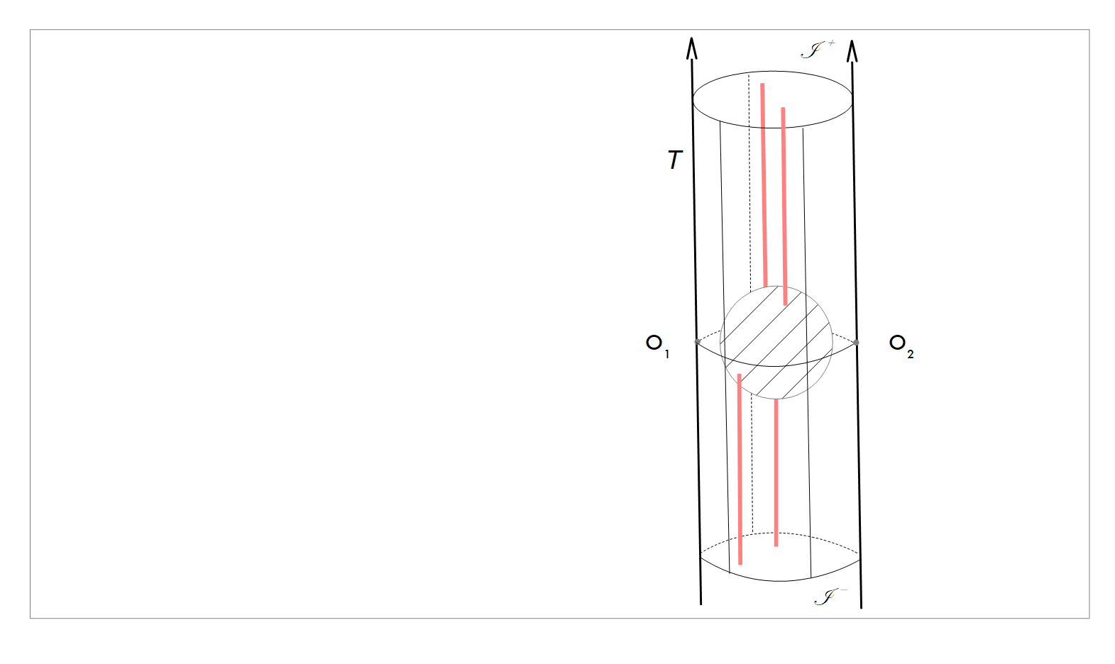
Another interesting avenue comes via a picture I stole from a talk by Laura Donnay on the Carrollian limit and flat space holography:

Stole this picture from a talk by Laura Donnay. The S-matrix in/out states on plus / minus null infinity (ℐ ⁺, ℐ ⁻ ) on the left and poles in the conformal operator products on the celestial sphere on the right.

Translating the left side of Donnay’s diagram into the right side of my diagram above, you get something that looks like an S-matrix diagram (and the “anything goes” blob in the middle is essentially “anything goes” in the pocket of elsewhere):

A possible way forward in the description of the “elsewhere” interpretation of quantum mechanics in the Carrollian limit in terms of an S-matrix?

Again, I don’t know if this will be a fruitful direction. I mostly just thought it was interesting and wanted to write down my notes.

Topological fluctuation theorem

There’s a tangential new development in the fluctuation theorem that may also be interesting — the topological fluctuation theorem (also here). It turns out that the paths used in the derivation of the original fluctuation theorems result in something that is essentially:

\(\displaystyle e^{n \Delta S_{0}} \sim \frac{P(+n)}{P(-n)}\)

where n is the topological winding number (around vortices in the paper). The thing is that interference in quantum mechanics generally comes in via “loops” in (real space) Feynman diagrams — things that are essentially topological. The quantum double slit experiment is the sum of a path through each slit and a loop that goes through both slits. If our “quantum” of entropy change from the distance change is Δx ~ n ℏ/mc the we have something that looks a lot like “old quantum theory”.

Anyway, I’m going to challenge myself by trying to make all of these musings more rigorous. Of course, at their heart, these musings are not really very different from the observation that the Schrodinger equation is a diffusion equation in imaginary time. The newer piece is the connection to the structure of Minkowski space. We are still lacking that moment where the factor of i sneaks in.

1. Not saying the work of these two is “hobbyist tinkering” though I aspire to be able to say the weird stuff Susskind says and be taken as seriously.

2. It’s more of a back of the envelope estimation scales than a real derivation.

3. The apparent reference is to the line: “My dear, here we must run as fast as we can, just to stay in place. And if you wish to go anywhere you must run twice as fast as that.”

4. It has been proposed that a “particle” should be defined in terms of a representation of the BMS group (the current “definition” — if there is one — is in terms of the Poincare group).

5. Note the additional factor of the speed of light in the Compton wavelength still means θ → 0 as c → 0, just “faster” since if ℓ ~ ℏ/mc then θ ~ c/ℓ = mc²/ℏ.